Tools for attribute-level importance and attendance in conjoint survey experiments — which attribute levels drive choices, how they rank, and which ones respondents ignore.
Why cjdiag?
Standard conjoint analysis tools (cjoint, cregg) estimate what respondents prefer — Average Marginal Component Effects (AMCEs) and marginal means. But they cannot tell you how respondents decide: which attributes they actually attend to, whether they process information hierarchically, or which attribute levels they ignore entirely.
cjdiag fills this gap with five diagnostic methods that reveal the decision process behind conjoint choices.
Installation
# Install from GitHub (CRAN submission pending)
# install.packages("pak")
pak::pak("dkarpa/cjdiag")
Quick Start
library(cjdiag)
data(immig)

rf <- cj_fit(
  Chosen_Immigrant ~ Gender + Education + LanguageSkills +
    CountryofOrigin + Job + JobExperience + JobPlans +
    ReasonforApplication + PriorEntry,
  data = immig,
  method = "forest"
)

rf
#> Conjoint Random Forest
#> ======================
#>
#> Resolution: levels
#> Trees: 500
#> OOB Error: 40.3%
#> Observations: 2,000
#> Attributes: 9
#> Levels: 50
#>
#> Top 10 levels by MDA:
#>
#> # A tibble: 10 × 7
#>     rank attribute       level                      mda root_pct class_0 class_1
#>    <int> <chr>           <chr>                    <dbl>    <dbl>   <dbl>   <dbl>
#>  1     1 JobPlans        no plans to look for wo… 13.5      15.4  12.3      7.25
#>  2     2 JobPlans        contract with employer    8.18     11.2   3.70     6.98
#>  3     3 Education       no formal                 7.87      7.4   8.04     2.38
#>  4     4 PriorEntry      once w/o authorization    7.42     10.4   6.87     3.66
#>  5     5 LanguageSkills  fluent English            6.16      8.2   2.71     6.00
#>  6     6 PriorEntry      once as tourist           4.83      2.4   1.61     5.25
#>  7     7 Education       college degree            4.75      6.4   0.153    6.16
#>  8     8 LanguageSkills  used interpreter          4.66      5.6   4.91     1.37
#>  9     9 CountryofOrigin Iraq                      4.15      4.6   3.53     2.15
#> 10    10 Job             janitor                   3.87      3     2.09     3.36
The full results table is the main output. Each row is one attribute level. The columns:
- rank — position in the importance ordering. Rank 1 = the level that does the most work in driving choices.
- attribute — the conjoint attribute (the question the level answers, e.g. what is this immigrant’s reason for applying?).
- level — the specific value of that attribute (e.g. escape persecution).
-
mda — Mean Decrease in Accuracy. How much the forest’s predictive accuracy drops when the information in this level is shuffled away. Higher = this level genuinely shapes choices. Levels with
mdanear zero are effectively ignored. - root_pct — % of trees in the forest where this level is the first split. A high value means respondents tend to start their decision by checking this level. This is the gatekeeper signal.
- class_0 — how strongly this level pushes respondents to reject a profile. A “veto” signal.
- class_1 — how strongly this level pushes them to select a profile. An “attractor” signal.
The asymmetry between class_0 and class_1 reveals direction. class_0 ≫ class_1 means the level is a deal-breaker (e.g. no plans to look for work mostly causes rejection). class_1 ≫ class_0 means the level is a draw (e.g. fluent English mostly causes selection).
knitr::kable(
  head(rf$results, 20)[, c("rank", "attribute", "level", "mda",
                           "root_pct", "class_0", "class_1")],
  digits = 2
)| rank | attribute | level | mda | root_pct | class_0 | class_1 |
|---|---|---|---|---|---|---|
| 1 | JobPlans | no plans to look for work | 13.48 | 15.4 | 12.33 | 7.25 |
| 2 | JobPlans | contract with employer | 8.18 | 11.2 | 3.70 | 6.98 |
| 3 | Education | no formal | 7.87 | 7.4 | 8.04 | 2.38 |
| 4 | PriorEntry | once w/o authorization | 7.42 | 10.4 | 6.87 | 3.66 |
| 5 | LanguageSkills | fluent English | 6.16 | 8.2 | 2.71 | 6.00 |
| 6 | PriorEntry | once as tourist | 4.83 | 2.4 | 1.61 | 5.25 |
| 7 | Education | college degree | 4.75 | 6.4 | 0.15 | 6.16 |
| 8 | LanguageSkills | used interpreter | 4.66 | 5.6 | 4.91 | 1.37 |
| 9 | CountryofOrigin | Iraq | 4.15 | 4.6 | 3.53 | 2.15 |
| 10 | Job | janitor | 3.87 | 3.0 | 2.09 | 3.36 |
| 11 | CountryofOrigin | Mexico | 3.34 | 0.2 | 1.41 | 3.47 |
| 12 | CountryofOrigin | Germany | 3.00 | 0.2 | 3.24 | 1.05 |
| 13 | LanguageSkills | broken English | 2.99 | 0.2 | -0.38 | 4.60 |
| 14 | JobPlans | will look for work | 2.84 | 0.0 | 2.04 | 1.55 |
| 15 | Job | doctor | 2.22 | 1.4 | 2.26 | 0.93 |
| 16 | PriorEntry | six months with family | 2.13 | 1.4 | 0.58 | 2.29 |
| 17 | LanguageSkills | tried English but unable | 1.90 | 0.4 | 2.28 | 0.26 |
| 18 | ReasonforApplication | reunite with family | 1.86 | 0.2 | 0.04 | 2.58 |
| 19 | Gender | male | 1.67 | 0.6 | 0.56 | 1.86 |
| 20 | ReasonforApplication | escape persecution | 1.45 | 1.0 | -2.40 | 4.24 |
Decision Tree
tr <- cj_fit(
  Chosen_Immigrant ~ Gender + Education + LanguageSkills +
    CountryofOrigin + Job + JobExperience + JobPlans +
    ReasonforApplication + PriorEntry,
  data = immig,
  method = "tree"
)

plot(tr)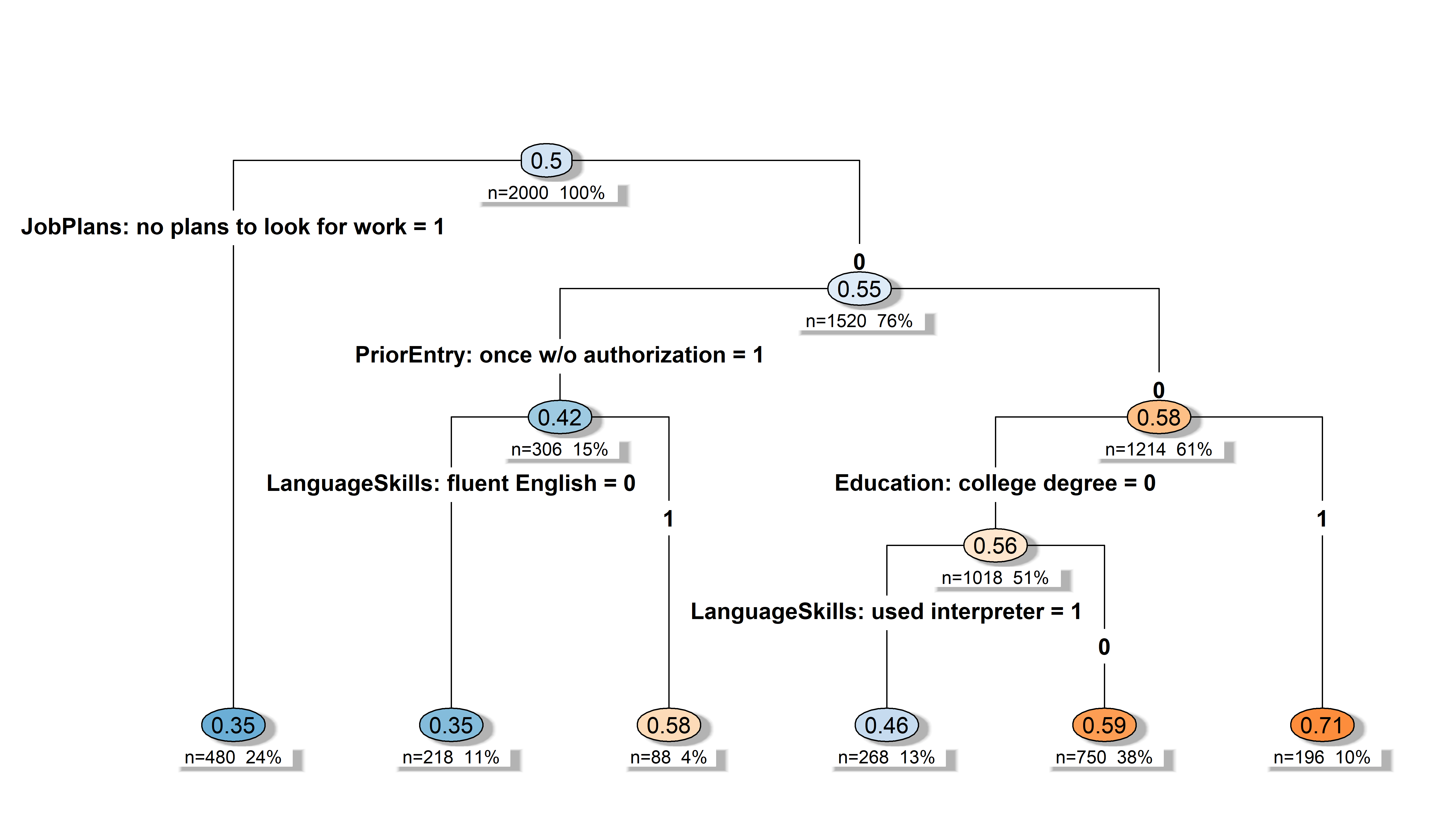
Nested Marginal Means
nmm <- cj_fit(
  Chosen_Immigrant ~ Gender + Education + LanguageSkills +
    CountryofOrigin + Job + JobExperience + JobPlans +
    ReasonforApplication + PriorEntry,
  data = immig,
  method = "nmm",
  resp_id = "CaseID",
  n_boot = 0
)

plot(nmm, type = "cumulative", top_n = 20)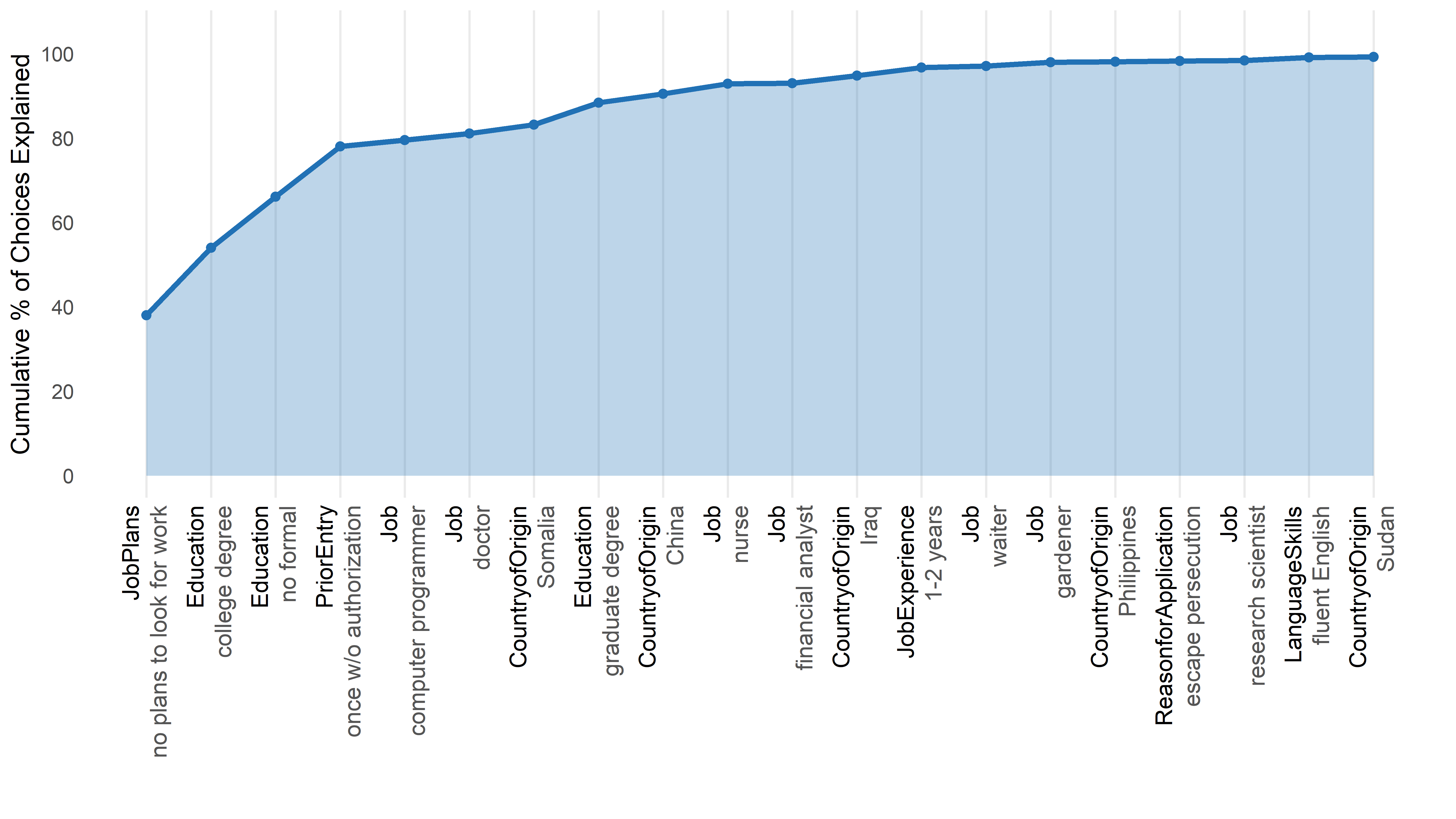
CRT Lambda-Survival
The CRT survival statistic — the largest L1 penalty at which a level’s coefficient is still nonzero — gives a one-number attendance ranking. Below, fit to HH15 with a grid up to 1000.
crt <- cj_fit(
  Chosen_Immigrant ~ Gender + Education + LanguageSkills +
    CountryofOrigin + Job + JobExperience + JobPlans +
    ReasonforApplication + PriorEntry,
  data = immig,
  method = "crt",
  lambda_grid = c(seq(25, 250, 25), seq(300, 500, 50), seq(600, 1000, 100))
)

plot(crt, type = "survival", top_n = 15)   # coefficient path
plot(crt, type = "rank")                    # connected-dot survival ranking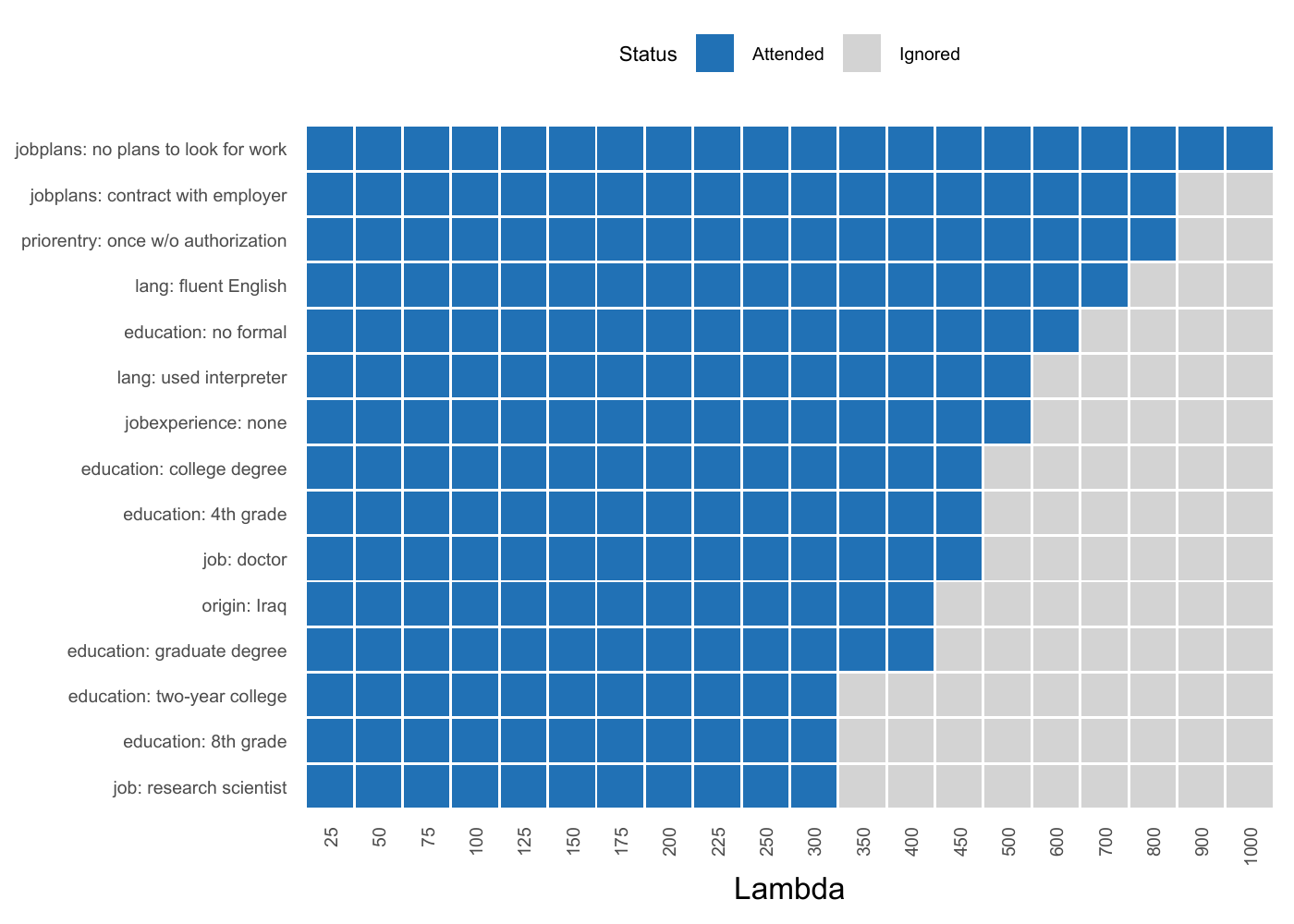
Methods
All methods are accessed through a single function: cj_fit(formula, data, method).
| Estimand | method = |
Question | Output | Behavioural assumption | When to use |
|---|---|---|---|---|---|
| Level importance | "forest" |
Which attribute levels matter most? | MDA, root-split rate per level | None — non-parametric | Default. Always fit this first. |
| Decision structure | "tree" |
How do respondents structure their decisions? | Hierarchical CART splits | Lexicographic / sequential | When you suspect a gatekeeper. |
| Level attendance | "crt" |
Which levels survive a strict signal-vs-noise test? | Lambda-survival, attended/ignored | Sparsity (most levels are noise) | When you want a hard attendance test. |
| Decision order | "nmm" |
In what order do levels settle choices? | Decisiveness ranking, cumulative % | Sequential elimination (EBA) | When you care about the decision order. |
| Individual attendance | "marginal_r2" |
Which attributes did each respondent actually use? | Per-respondent R² matrix | Per-respondent simple-regression fit | When you want individual-level heterogeneity. |
Plot Customization
All plot methods return ggplot2 objects and accept customization parameters:
# Colorblind-safe palette
plot(rf, palette = "colorblind")

# Rename attributes in display
plot(rf, attribute.names = c(LanguageSkills = "English Proficiency"))

# Full ggplot2 theme override
plot(rf, theme = ggplot2::theme_classic(base_size = 14))
Three palettes available: "default", "colorblind" (Okabe-Ito), "grey".
Set defaults once with set_cjdiag_theme() and set_cjdiag_labels().
Related Packages
cjdiag is complementary to packages that estimate AMCEs and design conjoint experiments:
- cjoint — AMCE estimation (Hainmueller, Hopkins & Yamamoto)
- cregg — AMCE and marginal means with tidy output
- projoint — full conjoint pipeline
- cbcTools — conjoint experiment design and power analysis
Run cjoint or cregg for AMCEs, then cjdiag to diagnose how respondents actually made those choices.
Getting Started
For a full walkthrough, see the Getting Started vignette. Each method has its own task-oriented vignette: forest, tree, nmm, marginal_r2, crt.
Citation
citation("cjdiag")Um Paket 'cjdiag' in Publikationen zu zitieren, nutzen Sie bitte:
Karpa D (2026). _cjdiag: Diagnostic Tools for Conjoint Survey
Experiments_. R package version 0.2.1,
<https://github.com/dkarpa/cjdiag>.
Ein BibTeX-Eintrag für LaTeX-Benutzer ist
@Manual{,
title = {cjdiag: Diagnostic Tools for Conjoint Survey Experiments},
author = {David Karpa},
year = {2026},
note = {R package version 0.2.1},
url = {https://github.com/dkarpa/cjdiag},
}Funding
David Karpa acknowledges financial support from the European Research Council (ERC) under the European Union’s Horizon Europe research and innovation programme — project AGAPP “Algorithmic Governance – A Public Perspective” (ERC Starting Grant, grant agreement No. 101116772, PI: Prof. Daria Gritsenko), where he works as a postdoctoral researcher.