When to use
Use method = "nmm" (Dill, Howlett & Mueller-Crepon
2024) when you care about the order in which attribute levels
settle choices, not just their static importance. NMM is the closest
match to elimination- by-aspects (Tversky 1972) at the level of
attribute levels.
The procedure works sequentially:
- Identify the level whose marginal mean deviates most from 50/50 — the most decisive level.
- Remove choice tasks where that level cannot discriminate (because both profiles share it).
- Repeat on the reduced sample.
The cumulative plot shows how quickly the top levels account for the total decisiveness.
Fit
nmm <- cj_fit(f, data = immig, method = "nmm",
              resp_id = "CaseID", n_boot = 0)
nmm
#> Conjoint Nested Marginal Means
#> ==============================
#>
#> Observations: 2,000
#> Attributes: 9
#> Levels: 50
#>
#> Total pairs: 1,000
#> After top 5: 205 (20.5% remaining)
#>
#> Top 10 levels by decisiveness:
#>
#> # A tibble: 10 × 6
#>     rank attribute       level                      mm decisiveness pct_of_total
#>    <int> <chr>           <chr>                   <dbl>        <dbl>        <dbl>
#>  1     1 JobPlans        no plans to look for w… 0.305        0.389         38
#>  2     2 Education       college degree          0.687        0.375         16
#>  3     3 Education       no formal               0.331        0.339         12.1
#>  4     4 PriorEntry      once w/o authorization  0.303        0.395         11.9
#>  5     5 Job             computer programmer     0.733        0.467          1.5
#>  6     6 Job             doctor                  0.688        0.375          1.6
#>  7     7 CountryofOrigin Somalia                 0.714        0.429          2.1
#>  8     8 Education       graduate degree         0.712        0.423          5.2
#>  9     9 CountryofOrigin China                   0.762        0.524          2.1
#> 10    10 Job             nurse                   0.667        0.333          2.4
Plot the cumulative explanation curve
plot(nmm, top_n = 20)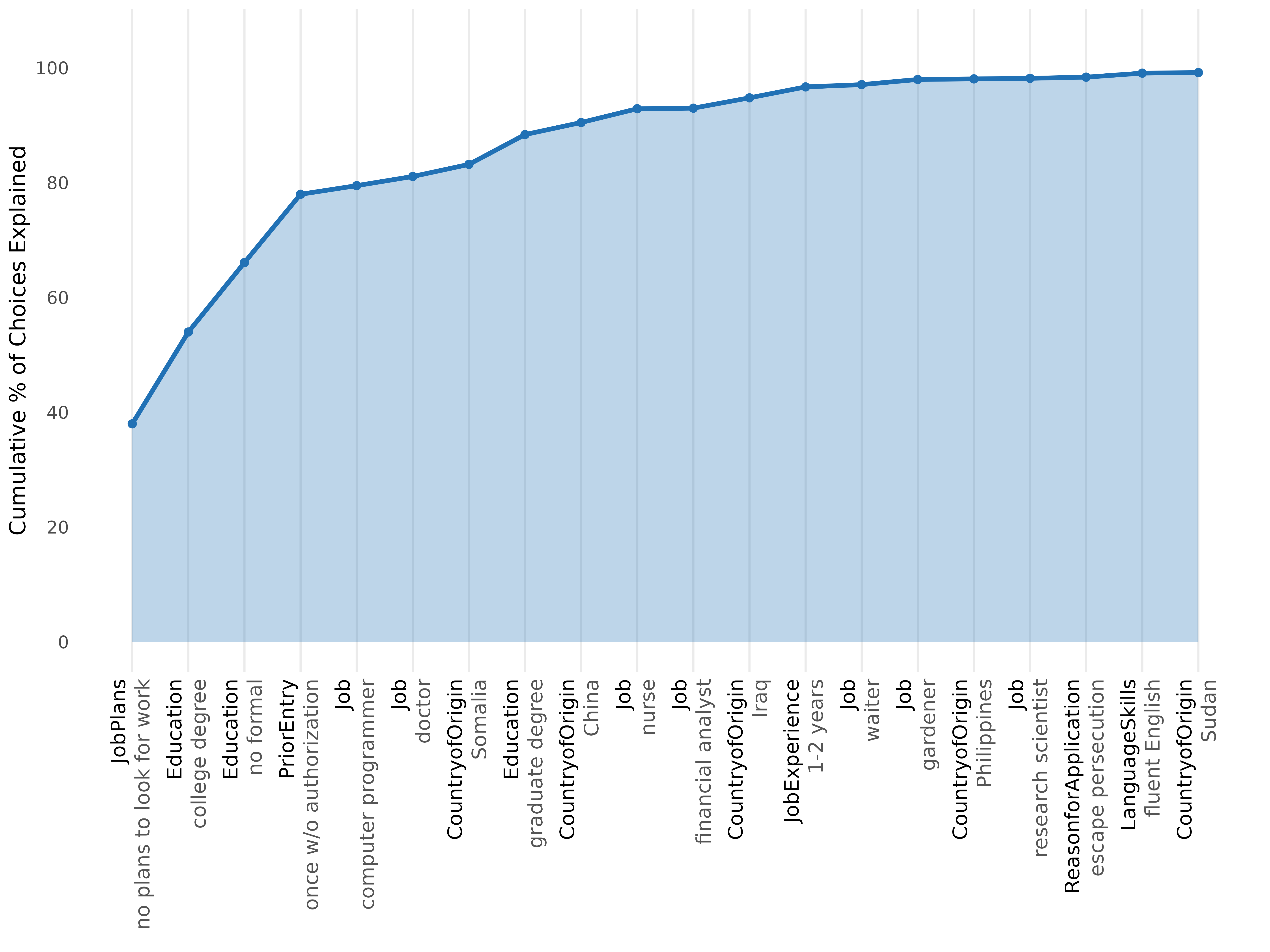
A steep early curve = a strong decision-order hierarchy: a few top-ranked levels settle most of the choices. A flat curve = compensatory processing, where many levels each contribute a little.
Related
- Decision Tree for an alternative hierarchical representation that uses CART splits instead of marginal means.
- Random Forest for static level importance without an ordering assumption.